Quantitative Methods Across Chapters
Dollar Value Figures
For analyses using IPUMS data in the tables below, negative or zero values for household income, rent, and home value were treated as missing. Rent burden and severe rent burden measures exclude households designated as “not computed” in the tables provided by the Census Bureau.
All dollar amounts are inflation-adjusted to be expressed in 2023 dollars, based on the Consumer Price Index (CPI).
Race and Ethnicity Definitions
All racial categories reported are non-Hispanic. For example, “White” refers to non-Hispanic White individuals, “Black” refers to non-Hispanic Black individuals, and so forth. The Hispanic/Latino category includes all individuals of Hispanic or Latino origin, regardless of race. Categories include:
- American Indian/Alaska Native (AIAN)
- Asian/Pacific Islander
- Black/African American
- Hispanic/Latino
- White
- Other
Age Categories
- Under 18
- 18 – 24
- 25 – 54
- 55 – 61
- 62 & Over
Aggregating Neighborhood Data
To adapt data from broader geographic scales down to the neighborhood level, we use a crosswalk that aggregates data across geographies based on relative areas. For this report, much of the data is presented at the neighborhood level but originates from the census tract level. The geospatial crosswalk process is performed in ArcGIS by importing census tract and neighborhood shapefiles, calculating the areas where the polygons intersect, and determining what share of each intersection belongs to the original tract and to the new neighborhood. This process allows us to estimate how much of each tract’s characteristics fall within each neighborhood.
The process varies depending on the type of measure:
Aggregate measures (such as counts) utilize the area share of the original geography (in this case, census tract). For example, if a tract has 1,000 people, and 70% of the tract falls in Glendale and 30% of the tract falls in Burbank, we estimate that 700 of these people live in Glendale and 300 of them live in Burbank.
Averages and medians utilize the population share of the new geography (in this case, neighborhood). For example, using the same tract, if the median household income is $100,000, we assign that same median to both subpopulations—700 people in Glendale and 300 in Burbank. These subpopulations are then combined with population-weighted values from all other tracts that make up each neighborhood.
LABarometer
LABarometer is an internet survey panel of approximately 2,000 individuals randomly selected from households throughout Los Angeles County. It has been in operation since 2019 and is a subpanel of the Understanding America Study (UAS), a national internet survey panel managed by the USC Dornsife Center for Economic and Social Research. Surveys are fielded to the LABarometer panel on a biannual basis to monitor social and economic conditions in L.A. County, with a focus on four key issues: livability, affordability, mobility, and sustainability. For more information about LABarometer, including up-to-date demographic information, recruitment and retainment procedures, standard variables, and survey weights, please visit the LABarometer website here.
Qualitative Insights
Planning Department Listening Sessions
In October 2024, Neighborhood Data for Social Change (NDSC) hosted two listening sessions with staff from eight Los Angeles County cities—Huntington Park, Santa Fe Springs, South Pasadena, South Gate, Pasadena, Rolling Hills Estates, San Fernando, and Bell. These sessions gathered qualitative input from local housing and planning officials on key priorities, challenges, and data needs. Participants discussed their experiences implementing state housing laws, balancing development types, addressing resident concerns, and coordinating with neighboring jurisdictions.
Developer Survey
The Lusk Center for Real Estate conducted a survey in August 2024 to learn about the attitudes of housing developers towards the current housing market in Los Angeles. The survey was distributed to residential real estate developers in Southern California that had previously attended the Lusk Center for Real Estate Casden Multifamily Forecast, an annual report about multifamily real estate trends across Southern California submarkets. The short, 10 minute Qualtrics survey was created by Lusk Center faculty affiliate Moussa Diop and the Neighborhood Data for Social Change team. It was distributed via email blast and garnered 27 respondents. Respondents received compensation of a $25 discount for registration to the annual USC Casden Multifamily Forecast.
Population Characteristics
Data Points
|
Dataset
|
Definition & Notes
|
Source
|
|---|---|---|
|
Total Population by Decade
|
The total number of people living in each decade from 1950 - 2010
|
1950 - 2010: Decennial Census (accessed through Social Explorer)
|
|
Foreign-Born Population by Decade
|
The number of people who were not born in the United States or Puerto Rico in each decade from 1950 - 2010
|
1970 - 2000: Decennial Census (accessed through Social Explorer) 2010: American Community Survey 1-year estimates Table B05001
|
|
Total Population by Year
|
The total number of people in each year from 2010 - 2023
|
2010- 2023: American Community Survey 1-year estimates Table B01003
|
|
Annual Births
|
The annual number of births to Los Angeles County residents (even if the birth did not take place in Los Angeles County)
|
2018 - 2023: California Department of Public Health
|
|
Annual Deaths
|
The annual number of deaths of Los Angeles County residents (even if the death did not take place in Los Angeles County)
|
2018 - 2023: California Department of Public Health
|
|
Foreign Born Population by Year
|
The number of people living in Los Angeles County, who were not born in the United States or Puerto Rico in each year from 2010 - 2023
|
2010- 2023: American Community Survey 1-year estimates Table B05001
|
|
Percent Change in Population Under 24
|
The percentage change in the percentage of the population that was younger than 24, between 2010 and 2023
|
2010 & 2023: American Community Survey 1-year estimates (Table DP05)
|
|
Percent Change in Population 62 & Over
|
The percentage change in the percentage of the population that was older than 62, between 2010 and 2023
|
2010 & 2023: American Community Survey 1-year estimates (Table DP05)
|
|
Number of Households by Tenure and Year
|
The number of households living in housing units, by the occupant type of the housing unit (owner occupied vs. renter occupied) in each year from 2010 - 2023
|
2015- 2023: American Community Survey 1-year estimates Table B25003
|
|
Households with One Resident
|
The share of households occupied by a single resident
|
2010 & 2023: American Community Survey 1-year estimates Table S1101
|
|
Families with Children
|
The share of households with a child under the age of 18 who is related to the head of household (by marriage, adoption or birth) living in the home.
|
2010 & 2023: American Community Survey 1-year estimates Table S1101
|
Housing Supply
Data Points
|
Dataset
|
Definition & Notes
|
Source
|
|---|---|---|
|
Average Annual Population Increase by Decade
|
The average number of people added to the population each year within a given decade
|
1950 & 1960: U.S. Department of Housing and Urban Development. (1966). Comprehensive Housing Market Analysis: Los Angeles, California. Office of Program Policy Development. https://www.huduser.gov/portal/publications/pdf/scanned/scan-chma-LACalifornia-1966.pdf 1970 - 2020: Decennial Census (accessed through Social Explorer)
|
|
Average Annual New Housing Units by Decade
|
The average number of housing units added to the population each year within a given decade
|
1950 & 1960: U.S. Department of Housing and Urban Development. (1966). Comprehensive Housing Market Analysis: Los Angeles, California. Office of Program Policy Development. https://www.huduser.gov/portal/publications/pdf/scanned/scan-chma-LACalifornia-1966.pdf 1970 - 2020: Decennial Census (accessed through Social Explorer)
|
|
Median Age of Housing by Tenure
|
The median year that the residential structures (renter and owner occupied) were built. Median age is calculated by subtracting the median year built from 2023. Age refers to when the building was first constructed, not when it was remodeled, added to, or converted. Housing units built prior to 1939 are coded simply as “1939.” As a result, this measure is most useful for analyzing new housing construction over the past 85 years, rather than distinguishing among housing built in earlier periods (e.g 1800s).
|
2023: American Community Survey 1-Year estimates (Table B25037)
|
|
New Units Certified by Tenure
|
The number of new housing units certified for occupancy, broken out by intended occupant (owner or renter)
|
2018 - 2024: See Current Trends in Countywide Housing Production methodology section below
|
|
New Units Certified by Affordability
|
The number of new housing units certified for occupancy, broken out by affordability for: VLI: Households making less than 50% of Area Median Income LI: Households making between 50 - 80% of Area Median Income MI: Households making between 80 - 120% of Area Median Income ABMI: Households making above 120% Area Median Income The U.S. Department of Housing and Urban Development (HUD) calculates Area Median Income (AMI) each year for counties and metropolitan areas across the United States. AMI represents the midpoint of a region’s income distribution—half of households earn more and half earn less—and is used to set income limits for housing programs, adjusted for household size and local cost of living.
|
2018 - 2024: See Current Trends in Countywide Housing Production methodology section below
|
|
New Units Certified by Structure Type
|
The number of new housing units certified for occupancy, broken out by the size of the building: - Accessory Dwelling Unit (ADU) - Single Family (Detached & Attached) - 2-4 Unit - 5+ Unit
|
2018 - 2024: See Current Trends in Countywide Housing Production methodology section below
|
|
New Housing Units per Capita
|
The number of new housing units certified for occupancy between 2018 and 2024 per 10,000 people in each jurisdiction
|
2018 - 2024: Certificates of Occupancy - see Current Trends in Countywide Housing Production methodology section below 2023: Population, American Community Survey 5-year estimates
|
|
New Units Certified for Occupancy vs. Regional Housing Needs Assessment Goals
|
The number of new housing units certified for occupancy between 2021 and 2024 The number of new housing units required by each jurisdiction’s 6th Cycle Regional Housing Needs Assessment
|
2021 - 2024: Certificates of Occupancy - see Current Trends in Countywide Housing Production methodology section below 6th Cycle Regional Housing Needs Assessment via Southern California Association of Governments (SCAG)
|
|
Total Number of Rental Units
|
Total number of rental housing units, a sum of renter occupied units, units vacant for rent and vacant units rented but not yet occupied
|
2023: American Community Survey 1-year estimates for countywide, and 5-year estimates for neighborhood-level aggregates Table B25003 and B25004
|
|
Average time from Permit to Occupancy (City of Los Angeles)
|
The average length of time, in months, between when a building permit is issued and when a completed housing unit receives its certificate of occupancy in the City of Los Angeles
|
Permits issued between 2018 and 2021 - see Current Trends in Countywide Housing Production methodology section below
|
|
Total Number of Subsidized Units
|
The estimated total number of subsidized or assisted units that receive at least one federal or state subsidy or program
|
2025: See Subsidized & Incentivized Housing methodology section below for the data sources
|
|
Total Number of Units in Subsidized Properties
|
The estimated total number of rental units in properties that receive at least one federal or state subsidy or program.
|
2025: See Subsidized & Incentivized Housing Data Sources section below
|
|
Total Number of Subsidized Properties
|
The estimated number of properties that receive at least one federal or state subsidy or program.
|
2025: See Subsidized & Incentivized Housing Data Sources section below
|
|
Share of Rental Units Located in Subsidized Properties
|
Total Number of Units in Subsidized Properties divided by Total Number of Rental Units
|
2025: numerator, see Subsidized & Incentivized Housing Data Sources section below 2023: denominator, American Community Survey 5-year estimates Table B25003 and B25004
|
|
Annual Permanent Housing Beds Available by Housing Type by Year
|
Total number of permanent housing beds that are in Permanent Supportive Housing, Rapid Rehousing, and other types of permanent housing
|
2017-2023: U.S. Department of Housing and Urban Development. Point-in-Time Count and Housing Inventory Count.
|
|
Housing Choice Voucher Families
|
Total number of renter families that use tenant-based Housing Choice Vouchers
|
2024: U.S. Department of Housing and Urban Development. Picture of Subsidized Households.
|
|
Permanent Housing Beds for People Experiencing Homelessness
|
The number of year-round beds in housing programs—such as Permanent Supportive Housing, Rapid Re-Housing, and other permanent housing models—that provide long-term, stable living arrangements for individuals and families exiting homelessness across all Continuums of Care in Los Angeles County.
|
2017 - 2024: U.S. Department of Housing and Urban Development Housing Inventory Count (HIC)
|
Current Trends in Countywide Housing Production
New Units Certified for Occupancy
Jurisdictions across Los Angeles County submit annual progress reports to the California Department of Housing and Community Development (HCD). This dataset is available for housing production across LA County from 2018 to 2024. While the dataset contains information on entitlements, permits, and certificates of occupancy, this report focuses on certificates of occupancy due to the verified reliability of this variable and to emphasize units that are ready to be used.The accuracy of this data depends on what each jurisdiction reports. The California Department of Housing and Community Development (HCD) does not systematically verify these submissions, and smaller cities may have limited capacity or resources to track and report data consistently.
This dataset contains duplicate rows for some projects, depending on how each individual jurisdiction logs each step of the process. For this step of the analysis, the dataset can be narrowed down to rows where the year submitted is identical to the year of the certificate of occupancy date. For example, the following rows represent the same project that may appear twice:
| project_id | year | entitlement_date | permit_date | completion_date |
| ADU-1519189 | 2022 | . | 6/1/2022 | 1/1/2023 |
| ADU-1519189 | 2023 | . | . | 1/1/2023 |
To ensure this project is counted as a completed unit exactly once, the first row (which was logged during the permit date, but had the completion date retroactively updated) is ignored. Final totals for certificate of occupancy are directly verified against the HCD Data Dashboard as of 8/6/2025.
Average Time from Permit to Completion (City of Los Angeles Only)
This portion of the analysis is limited to the City of Los Angeles. Analyzing longitudinal timelines from permit to completion requires additional cleaning to individual rows of data. We focus on permits and certificates of occupancy for this analysis because entitlement dates are not fully available for the majority of properties in this dataset. The objective of this step is to have each development project appear as exactly one row, with all of the pertinent information filled in. Some jurisdictions retroactively fill in dates for projects and thus are ready for longitudinal analysis (Example 1). Others record new rows for each step of the process (Example 2), and thus need to be matched on the identifying fields – Assessor’s Parcel Number and “project tracking ID” (often a building permit number).
Example 1: Steps are recorded cumulatively, ready for timeline analysis
project_id | Assessor’s Parcel Number (APN) | year | entitlement_date | permit_date | completion_date |
ADU-1519189 | 123-456-7890 | 2019 | 1/1/2018 | 6/1/2018 | 2/1/2019 |
Example 2: Each step is recorded exactly once; need to be combined into one row by matching on unique ID
project_id | Assessor’s Parcel Number (APN) | year | entitlement_date | permit_date | completion_date |
ADU-1519189 | 123-456-7890 | 2018 | 1/1/2018 | . | . |
ADU-1519189 | 123-456-7890 | 2018 | . | 6/1/2018 | . |
ADU-1519189 | 123-456-7890 | 2019 | . | . | 2/1/2019 |
In order to merge as many properties as possible, the following steps were taken to clean the matching fields:
- Removed special characters
- Converted all characters to lower cases
- Replaced obviously not unique tracking IDs with blanks
Projects with blank project tracking IDs were omitted, since it is impossible to know if they can be matched with another project in the dataset or not. We also ignored rows that reported inconsistent numbers of units in the permitting step of the process, since it is unreliable to have a different unit count in the middle step of the process (ex. 4 entitlements reported, 1 permit reported, and 4 certificates of occupancy reported).
For properties in the data that matched, some displayed differing dates for permitting or completion that need to be fixed before properties can be merged together. First, we cross-checked permit and certificate of occupancy data in the Housing Element dataset with a public dataset provided by the Los Angeles Department of Building and Safety (LADBS), and corrected dates in the Housing Element dataset when necessary. Looking at instances where the same property still had different dates recorded, there were 2 cases for permit dates and 3,876 cases for certificates of occupancy. For these rows, we replaced the existing dates with the average value of the two dates.
Once all of the properties are matched together, the analysis ignores properties where the certificate of occupancy date was before permit date. The analysis also ignores properties where the permit date and certificate of occupancy date are less than a month apart. This is unlikely to accurately reflect the time between the steps of this process.
Our analysis references average time spans for housing development in Los Angeles. We have provided medians as well in the tables below, for reference.
Average Time from Date of Permit → Date of Completion | Median Time from Date of Permit → Date of Completion | ||
All Units | Total | 18 months (17 months, 21 days) | 14 months, 2 days |
By tenure: | Owner-Occupied | 20 months (20 months, 1 day) | 16 months, 9 days |
Renter-Occupied | 17 months (17 months, 6 days) | 13 months, 17 days | |
By unit category | Accessory Dwelling Units | 17 months (16 months, 20 days) | 13 months, 8 days |
Single Family (detached) | 20 months (19 months, 23 days) | 16 months, 2 days | |
2 to 4 units | 16 months (16 months, 2 days) | 12 months, 28 days | |
5+ units | 35 months (34 months, 23 days) | 33 months, 16 days |
|
|
Average time from date of permit → Date of Completion
|
Median time from date of Permit → date of Completion
|
|---|---|---|
|
Affordable, 2-4
|
19 months, 18 days
|
21 months
|
|
Affordable, 5+
|
33 months, 13 days
|
32 months, 13 days
|
|
Market Rate, 2-4
|
16 months, 1 day
|
12 months, 28 days
|
|
Market Rate, 5+
|
34 months, 18 days
|
33 months, 8 days
|
Subsidized Housing
Data Sources
We compiled multiple sources of housing subsidy data to compile the list of residential properties with at least one active subsidy or project-based affordable housing program status, as of June 2025. Our main data sources include:
- United States Department of Housing and Urban Development (HUD)
- Insured Mortgages, limited to Section 221(d)(3), Section 221(d)(4), Section 236, and Section 202 financing
- Multifamily Assistance & Section 8 Database, including Project Rental Assistance Contract, Section 202/8, Project-Based Section 8, Section 8 – Rental Assistance Demonstration, Loan Management Set-Aside, etc.
- Low Income Housing Tax Credit (LIHTC)
- National Housing Preservation Database and Housing Authority of the City of Los Angeles (HACLA)
- Public Housing
- California Tax Credit Allocation Committee (CTCAC)’s LIHTC data
- California Housing Financing Agency (CalHFA)’s Mental Health Program, Mixed-Income Program, California Debt Limit Allocation Committee Tax Exempt Bond Special Needs Housing Program, and CalHFA-monitored Project-based Section 8
- California Department of Housing and Community Development (HCD)’s asset management portfolio, including properties with the following programs
- Affordable Housing and Sustainable Communities Program
- California Housing Rehabilitation Program
- Deferred Payment Rehabilitation Loan Program
- Family Housing Demonstration Program
- HOME Investment Partnerships Program
- Homeless Youth Multifamily Housing Program
- Housing for a Healthy California Program
- Infill Infrastructure Grant Program
- Multifamily Housing Program
- Multifamily Housing Program – Downtown Rebound Program
- Multifamily Housing Program – Governor’s Homeless Initiative
- National Housing Trust Fund Program
- Neighborhood Stabilization Program
- No Place Like Home Program
- Rental Housing Construction Program
- Special User Housing Rehabilitation Program
- State Earthquake Rehabilitation Assistance Program
- Supportive Housing Multifamily Housing Program
- Transit-Oriented Development Housing Program
- Veterans Housing and Homelessness Prevention Program
- Los Angeles Housing Department’s (LAHD) Affordable and Accessible Housing Registry website
Property-Level Data Compilation
Property-level data linkage and cleaning are crucial for understanding the subsidized and income-restricted housing stock. This is because a single property or development can leverage multiple subsidy sources to help develop affordable homes, and it is important to avoid overcounting the number of properties and units by simply adding the numbers up across programs (Reina & Williams, 2012). Kim and Eisenlohr (2022) present a detailed case study of an affordable housing development, showing how multiple subsidy programs were layered to structure the project’s financing, in conjunction with Community Land Trust.
We follow similar concepts and steps to the method used in the New York University Furman Center’s Subsidized Database to perform data linkage. As several data sources report the subsidy information at the development level, which sometimes can contain multiple addresses, we first separate multiple addresses to generate an address-level data set. For any invalid address, such as an intersection of two streets, we use the property information, such as the development name, to get the real address. Then, we standardized and cleaned the address text fields using the ArcGIS worldwide geocoder to get a preliminary spatial coordinate of the property. For addresses that fail to geocode or have a low match score, we manually look up the coordinates using Google Maps. We match the properties with the exact address text field. However, sometimes a property can have a range of house numbers or an alternative address on file; we need to take further steps to consolidate these addresses pointing to the same property. We use the following methods to perform the fuzzy match: 1) a spatial join of the property coordinates to the assessor’s parcel data to get the nearest parcel matched to the property address, and 2) address coordinates within 10 meters of each other. We then manually look up these addresses on the LA County Assessor’s portal and use web search to curate the property address crosswalk to prevent over-linkage.
Some of the developments can have scattered sites and sometimes be located across several neighborhoods, but many of these data sources only report the total number of units at the development level. To provide accurate estimates at the neighborhood level, we attempted to disaggregate the number of units in these scattered sites. If developments come with scattered site addresses but no property-level unit counts, we use LAHD’s AAHR listing, CTCAC’s development staff memo, LA County Assessor’s portal, and developer or property management’s website, PropertyShark, and Redfin data (order here representing the priority) to estimate the total number of units in these properties. We also cross-reference the total unit count across different data sources to help identify properties that are likely to be associated with a development with scattered sites.
Data Limitations
- Program coverage: We are still working on integrating local housing program information. The analysis is restricted to the federal or state-level programs, though some of these properties are cross-subsidized by local programs.
- Total number of units in subsidized properties: The total number of units reported in the analysis can contain market-rate units or units for property managers.
- Subsidized properties could include Permanent Supportive Housing (PSH). We use HUD’s Housing Inventory Count (HIC) data to determine the availability of permanent housing in LA County. We are only able to reliably identify half of the addresses in the HIC universe. The addresses that we are not able to geocode and link to the rest of the subsidized property data could be due to scattered sites, addresses pointing to government agencies, non-profit organizations, PO Boxes, etc. As we cannot systematically identify permanent housing in the subsidized properties for now, we have decided to include them in data reporting.
Homeowners
Data Points
|
dataset
|
definition & notes
|
Source
|
|---|---|---|
|
Homeownership Rate
|
The percentage of housing units occupied by the owner of the unit
|
1970 - 2020: Decennial Census (accessed through Social Explorer) 2022 - 2023: American Community Survey 1-Year Estimates Table B25003
|
|
Median Home Value
|
The median value of owner-occupied homes in Los Angeles City, Los Angeles County, California, and the United States, measured in 2023 dollars. Value is captured by asking the head of household’s estimate of how much the property (house and lot, mobile home and lot (if lot owned), or condominium unit) would sell for if it were for sale.
|
1980: Decennial Census (accessed through Social Explorer) 2023: American Community Survey 1-Year Estimates Table B25097
|
|
Median Household Income
|
The middle value for household income in Los Angeles City, Los Angeles County, California, and the United States, measured in 2023 dollars. Income is defined as any money that a person earns from work, selling products or services, or any other streams such as Social Security payments, pensions, child support, public assistance, annuities, money derived from rental properties, interest and dividends, etc.
|
1980: Decennial Census (accessed through Social Explorer) 2023: American Community Survey 1-Year Estimates Table B25119
|
|
Time Since Move In
|
The share of homeowner households who have been living in their homes for more than 20 years
|
2010 & 2023: American Community Survey 1-year estimates, accessed via IPUMS
|
|
Mortgage Status by Age of Householder & Household Income
|
Analysis of the share of homeowners who are under the age of 44 with and without a mortgage across various income levels
|
2010 & 2023: American Community Survey 1-year estimates, accessed via IPUMS
|
|
Homeownership Rates by Income
|
The percentage of housing units occupied by the owner of the unit, across households with the following incomes: under $50,000; $50,000 to $99,999; $100,000 to $149,999; $150,000 and over. Los Angeles County’s population is rapidly aging/retiring and older adults are significantly more likely to be homeowners. As aging homeowners retire and move into lower income categories, it may cause homeownership rates in lower income categories to appear as if they are rising, when in fact, existing homeowners are just retiring. In order to avoid this trend in the data, this analysis of homeownership rates by income is limited to households where the head of household is considered “of prime working age” (between the ages of 25 and 54).
|
2010 & 2023: American Community Survey 1-year estimates, accessed via IPUMS
|
|
Homeownership Rates by Race/Ethnicity
|
The percentage of housing units occupied by the owner of the unit among households headed by a person who identifies as the following racial/ethnic groups: American Indian Alaska Native, Asian/Pacific Islander, Black/African American, Hispanic/Latino, White, and Other
|
2010 & 2023: American Community Survey 1-year estimates, accessed via IPUMS
|
|
Homeownership Rates by Neighborhood
|
The percentage of housing units occupied by the owner of the unit, at the level of the neighborhood.
|
2023: American Community Survey 5-year estimates Table B25003
|
Homeownership Rates in Formerly Redlined Communities
This analysis examines whether present-day homeownership rates in Los Angeles City are correlated with historical “grades” assigned under the redlining policies of the federal government’s Home Owners’ Loan Corporation (HOLC) between 1935 and 1940.
We use Meier and Mitchell’s (2025) crosswalk data, which overlays 2020 Census Tracts on the HOLC maps and assigns to each tract a numerical value that reflects the degree of redlining the area faced. Since a single tract can overlap multiple, differently graded, HOLC zones, this score, ranging from 1 to 4, reflects the weighted average of the different grades applicable to each tract. The authors provide both a continuous score and a rounded, equal interval score. We make use of the latter in our analysis. A score of 1 represents an “A” grade, 2 represents “B”, 3 indicates “C” and 4, “D”.
In the present analysis we merge Census Tract-level data on the number of homeowner households (homeownership count) and the number of households of all tenure types (all households) to Meier and Mitchell’s crosswalk data, and collapse the merged dataset by HOLC grade to arrive at the sums of homeownership count and all households by grade. We then calculate the percentage of homeownership by grade as:
Citations
Nelson, R. K., Winling, L, et al. (2023). Mapping Inequality: Redlining in New Deal America. Digital Scholarship Lab. https://dsl.richmond.edu/panorama/redlining.
Meier, H. C. S. & Mitchell, B. C. (2025). Historic Redlining Indicator for 2000, 2010, and 2020 US Census Tracts (Version No. 3). Inter-university Consortium for Political and Social Research. https://www.openicpsr.org/openicpsr/project/141121/version/V3/view
Renters
Data Points
|
Dataset
|
Definition & Notes
|
Source
|
|---|---|---|
|
Rent Burden in the 10 Largest U.S. Metro Areas
|
The percentage of renters paying more than 30 percent of their monthly income on rent and utilities. 10 largest Metropolitan Statistical Areas (MSAs) based on 2020 Census data, including New York-Newark, Los Angeles-Long Beach-Anaheim, Chicago-Naperville-Elgin, Dallas-Fort Worth-Arlington, Houston-Pasadena-The Woodlands, Miami-Fort Lauderdale-West Palm Beach, Washington-Arlington-Alexandria, Atlanta-Sandy Springs-Roswell, Philadelphia-Camden-Wilmington
|
2023: American Community Survey 1-year estimates accessed from 2025 State of the Nation’s Housing, Joint Center for Housing Studies of Harvard University
|
|
Median Renter Income
|
The middle value of income of households occupied by renters in an area, measured in 2023 dollars Income is defined as any money that a person earns from work, selling products or services, or any other streams such as Social Security payments, pensions, child support, public assistance, annuities, money derived from rental properties, interest and dividends, etc.
|
1980 - 1990: Decennial Census accessed through IPUMS 2000: Decennial Census accessed through Social Explorer 2010, 2019 & 2023: American Community Survey 1-Year Estimates Table B25119
|
|
Median Gross Rent
|
The median value of gross rent prices in an area, measured in 2023 dollars. Gross rent is the rent price shown on the lease plus the estimated average monthly cost of utilities (electricity, gas, and water and sewer) and fuels (oil, coal, kerosene, wood, etc.) if these are paid by the renter.
|
1980 - 2000: Decennial Census (accessed through Social Explorer) 2010, 2019 & 2023: American Community Survey 1-Year Estimates Table B25064
|
|
Rent Burden
|
The percentage of renters paying more than 30 percent of their monthly income on rent and utilities
|
1980 - 2000: Decennial Census accessed through IPUMS 2010, 2019 & 2023: American Community Survey 1-Year Estimates Table B25070
|
|
Severe Rent Burden
|
The percentage of renters paying more than 50 percent of their monthly income on rent and utilities
|
1980 - 2000: Decennial Census accessed through IPUMS 2010, 2019 & 2023: American Community Survey 1-Year Estimates Table B25070
|
|
Renter Income Levels
|
The share of renter households with incomes in the following groups: under $50,000; $50,000 to $99,999; $100,000 to $149,999; $150,000 and over
|
2010 - 2023: American Community Survey 1-year estimates, accessed via IPUMS
|
|
Gross Rent Levels
|
Households that are paying rent in the following buckets: below $1250, $1250 to $2499, $2500 to $3749, $3750 and above
|
2023: American Community Survey 1-year estimates, accessed via IPUMS
|
|
Rent Burden by Income Level
|
The percentage of renters paying more than 30 percent of their monthly income on rent and utilities, across households with the following incomes: under $50,000; $50,000 to $99,999; $100,000 to $149,999; $150,000 and over
|
2011 & 2023: American Community Survey 1-year estimates, accessed via IPUMS
|
|
Severe Rent Burden by Income Level
|
The percentage of renters paying more than 50 percent of their monthly income on rent and utilities, across households with the following incomes: under $50,000; $50,000 to $99,999; $100,000 to $149,999; $150,000 and over
|
2011 & 2023: American Community Survey 1-year estimates, accessed via IPUMS
|
|
Rent Burden by Income by Neighborhood
|
The share of households with a household income of less than $100,000 who are paying more than 30% of their income on rent and utilities by neighborhood. Neighborhoods with less than 500 renter households making under $100,000 are excluded.
|
2023: American Community Survey 5-year estimates (B25074)
|
|
Rent Burden by Race/Ethnicity
|
The percentage of renters paying more than 30 percent of their monthly income on rent and utilities, among households headed by a person who identifies as the following racial/ethnic groups: Asian/Pacific Islander, Black, Hispanic/Latino, White
|
2011, 2019 & 2023: American Community Survey 1-year estimates, accessed via IPUMS
|
|
Severe Rent Burden by Race/Ethnicity
|
The percentage of renters paying more than 50 percent of their monthly income on rent and utilities, among households headed by a person who identifies as the following racial/ethnic groups: Asian/Pacific Islander, Black, Hispanic/Latino, White
|
2011, 2019 & 2023: American Community Survey 1-year estimates, accessed via IPUMS
|
|
Median Renter Income by Race/Ethnicity
|
The middle value of income of renter-occupied households in an area, measured in 2023 dollars, among households headed by a person who identifies as the following racial/ethnic groups: Asian/Pacific Islander, Black, Hispanic/Latino, White
|
2011 & 2023: American Community Survey 1-year estimates, accessed via IPUMS
|
|
Older Adult Renter Households
|
Households headed by a person ages 62 and older who are renting their homes
|
2010 & 2023: American Community Survey 1-year estimates, accessed via IPUMS
|
|
Rent Burden among Older Adults
|
The percentage of renters paying more than 30 percent of their monthly income on rent and utilities among households headed by a person ages 62 and older
|
2023: American Community Survey 1-year estimates, accessed via IPUMS
|
|
Severe Rent Burden among Older Adults
|
The percentage of renters paying more than 50 percent of their monthly income on rent and utilities among households headed by a person ages 62 and older
|
2023: American Community Survey 1-year estimates, accessed via IPUMS
|
Houseless Angelenos
Los Angeles County Continuum of Care (CoC) Homeless Count Methods
The LA CoC Homeless Count is conducted annually in an ongoing partnership between the University of Southern California (USC) and the Los Angeles Homeless Services Authority (LAHSA) since 2017. The Homeless Count provides a point-in-time (PIT) estimate of the unhoused population residing within the LA CoC geographic region, which is divided into eight Service Planning Areas (SPAs), including estimates of the sheltered and unsheltered populations. The LA CoC encompasses the whole of LA County, except for the cities of Pasadena, Glendale, and Long Beach who conduct their own respective PIT counts. Estimates of the unhoused population are derived from several data elements, including: 1) an observation-based count by volunteers of unsheltered individuals and dwellings (i.e., cars, vans, RVs, tents, and makeshift shelters), 2) a demographic survey of unsheltered adults (aged 25 years and older) conducted by a team at the USC Suzanne Dworak-Peck School of Social Work, 3) a youth survey-based count of unsheltered youth (aged 24 years and younger) mainly carried out by homelessness youth service provider agencies, and 4) a shelter count based on administrative data from the Homeless Management Information System (HMIS) and reporting from shelters not represented in HMIS. A detailed description of the LA CoC Homeless Count methodology can be found here. Here, we briefly describe each of the data elements and the general methodology used to arrive at the count of sheltered individuals and estimates of unsheltered individuals.
Point-in-Time Count: LAHSA conducts the PIT Count every January that can be thought of as measuring the visual homelessness in LAC CoC in that volunteers record their observations of the number of people they see living on the streets and dwellings assumed to be housing homeless individuals encountered while canvassing all 2,310 census tracts (CTs) that makeup the LA CoC. The counts for individuals encountered on the street are provided by estimated age category (under 18, 18 to 24, and 25 and older), with families counted separately from individuals.
Demographic Survey: Because the observations made by volunteers does not provide information about the number of people living in the dwellings that are counted or about the demographic characteristics the unsheltered population, the USC team conducts a separate survey between December and March each year across a sample of CTs in LA CoC using a two-stage stratified random sample approach. A team of data collectors canvass each sampled CT at least once during the surveying period and conduct surveys among any individual experiencing unsheltered homelessness they locate and who agrees to participate. The respondents are assumed to be selected at random from the homeless population in the CT. The survey collects information on basic demographic characteristics (i.e., age, gender, race/ethnicity), where the respondent slept last night and in the last 30 days, homelessness history, veteran status, health status, employment status, and more. Responses to the Demographic Survey are used to estimate the number of homeless individuals classified within select demographic and subpopulation categories. Proportions of individuals representing specific demographic and subpopulation characteristics are estimated within each household type (i.e., adults with children, adults without children, veterans without children, and veterans with children). These proportions are then applied to their respective PIT population totals at the SPA-level and then summed across SPAs to derive the estimated subpopulation counts for the CoC. Further, weights are used to estimate proportions from the survey data to account for the sampling method used. Sampling weights are applied to each demographic survey respondent, first calculated by taking the inverse probability of CT selection (for the CT where they were surveyed) and then adjusted to account for non-response and individuals who could not be approached (e.g., due to safety concerns) and post-stratified to the household PIT Count.
Youth Enumeration Survey: Homeless youth are considered a “hidden population” who may not be easily discernible through a visual tally. Therefore, survey-based methods are recommended to separately conduct a homeless youth count. The LA CoC Homeless Count utilizes a youth enumeration survey, collecting information on demographic characteristics and household composition, to estimate the size of the population under 25 years of age experiencing unsheltered homelessness and serve as a PIT count of unsheltered youth. To further describe the unsheltered youth population (e.g., veteran status, chronic homelessness status), data from the Demographic Survey conducted among individuals aged less than 25 years are used. The youth enumeration survey is typically conducted during the last 10 days of January across a selected sample of CTs within the LA CoC. Youth count efforts then employ three types of location-based data collection strategies to specifically target homeless youth: 1) street survey teams who canvass selected CTs and survey any identified youth-aged person experiencing homelessness willing to participate; 2) in-person surveys at survey sites (e.g., youth service providers); and 3) phone-based surveys at survey sites. Total, demographic, and subpopulation counts were calculated from the youth surveys by household type (i.e., unaccompanied transition aged youth and minors and parenting youth) using a similar method to the unsheltered adult count. The main difference in the methodology between the youth and adult unsheltered counts is that the adult unsheltered count is based on observations mostly by volunteers of individuals and CVRTM with complete coverage of the CoC, while the youth count is based on the Youth Enumeration Surveys conducted in a sample of CTs mostly by homeless youth service providers. This means that the sampling weights play a greater role in determining the number of unsheltered homeless youth. Youth sampling weights were calculated for the enumeration surveys as the inverse probability of selection and then adjusted for non-response. The enumeration survey was used to estimate basic demographic characteristics by household type and SPA, and the demographic survey was used to produce subpopulation proportions by household type and SPA.
Shelter Count: Shelter count estimates were generated using PIT shelter count data provided by LAHSA, which is a complete enumeration of all shelters in the LA CoC. The shelter PIT Count provides the raw number of homeless individuals living in emergency shelters, transitional housing, and safe havens, including those receiving vouchers for hotels or motels provided by these shelters. HMIS data is then used to estimate demographic and other subpopulation characteristics of sheltered individuals. HMIS data are assumed to be a complete enumeration of the sheltered population and, therefore, do not require additional weighting to generate demographic and subpopulation estimates. Demographic and subpopulation characteristics are derived by estimating the proportion within the HMIS data for each shelter type and household type (i.e., individuals, adult, and transition aged youth families and veterans). Proportions are then applied to the analogous PIT shelter household and individual counts, by household and shelter type, to obtain their characteristics. Subpopulation estimates are applied at the SPA level to SPA-specific counts and then summed to get the total CoC result.
Featured Chapter
Data Points
|
Dataset
|
Definition & Notes
|
Source
|
|---|---|---|
|
Total Number of Renter and Homeowner Households
|
Total number of renter households and homeowner households.
|
2023: American Community Survey 1-year estimates, accessed via IPUMS
|
|
Population Share by Race/Ethnicity
|
The percentage of the population identifying as Asian, Black/African American, Hispanic/Latino(a), White, and Other
|
2023: American Community Survey 5-year estimates Table B03002
|
|
Age Distribution
|
The percentage of population in the following age groups: below 18, 18-24, 25-34, 35-44, 45-54, 55-64, and 65 and above
|
2023: American Community Survey 5-year estimates Table B01001
|
|
Employment Status
|
The percentage of people in the civilian labor force who are employed
|
2023: American Community Survey 5-year estimates Table B23001
|
|
Homeownership
|
The percentage of housing units occupied by the owner of the unit
|
2023: American Community Survey 5-year estimates Table B25003
|
|
Median Household Income
|
The middle value for household income in an area, measured in 2023 dollars.
|
2023: American Community Survey 5-year estimates Table B19013
|
|
Average Household Size
|
The average number of people living in a household.
|
2023: American Community Survey 5-year estimates Table B25010
|
|
Living Arrangement, Share Young Adults Living with Parents
|
The percentage of adults living with child(ren) of the householder.
|
2023: American Community Survey 5-year estimates Table B09021
|
Methodology
For our analysis in the feature chapter, we partnered with LABarometer, a research center housed at the USC Dornsife Center for Economic and Social Research. Since 2019, LABarometer has run a biannual survey panel, designed to represent the diverse household mix of Los Angeles County and drawn from the Understanding America Study. The panel surveys approximately 2,000 randomly selected adults in each way to track changes in the county’s social and economic conditions. Details about how participants are selected and recruited can be found on LABarometer’s website (link).
The data we use comes from the Wave 3 Livability & Affordability Survey, conducted from June 6, 2022, to September 4, 2022. This survey collected detailed information to estimate how likely people are to change their housing status—specifically, to move from renting to owning or from owning to renting—based on their demographic and household characteristics. Out of 1,561 invited LA County residents, 1,139 completed the survey, yielding a response rate of nearly 73%.
By comparing answers from Wave 3 to those from later survey waves, LABarometer tracked whether respondents experienced a housing status shift. Respondents who participated in the Wave 3 survey but did not complete any subsequent survey waves, and observations that perfectly predict the outcome variable, are excluded from the analysis. The LABarometer team conducted Ordinary Least Squares (OLS) and logistic regression estimations to study how demographic and household factors influence the odds of transitioning between renting and owning a home. The chart below shows the sample sizes used for each regression model.
Table X: Sample sizes of regression analyses
|
Dependent Variable
|
ols
|
logistic regression
|
|---|---|---|
|
Transition from Renter into Homeowner
|
438
|
422
|
|
Transition from Homeowner into Renter
|
468
|
432
|
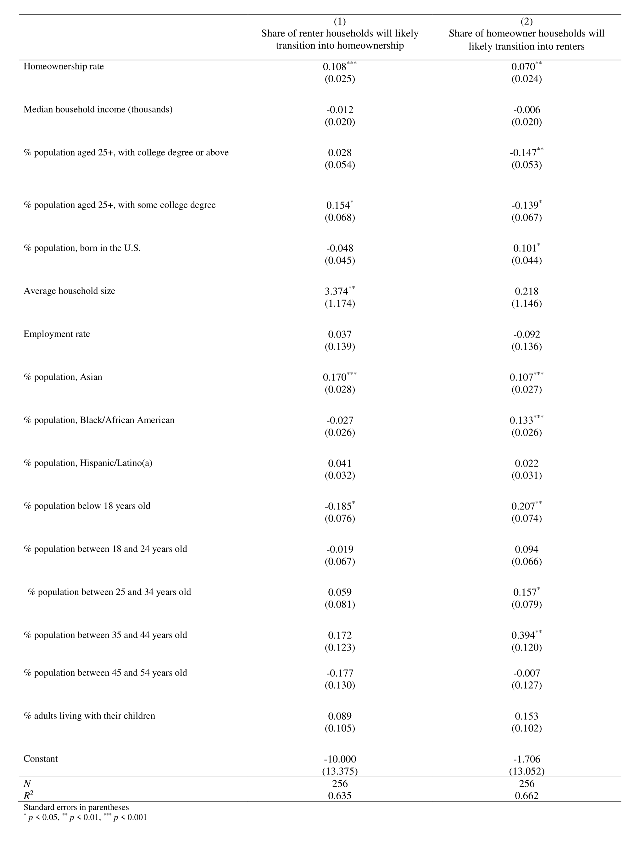
The OLS regression specification is:
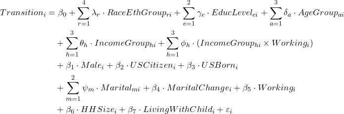
Where:
- i: respondent i.
- Transitioni: An indicator variable equal to 1 if respondent i transitioned from renting to owning (or vice versa), and 0 otherwise.
- RaceEthGroupri: a set of indicator variables identifying if respondent i is Black/African American, Asian, Hispanic, or another race/ethnicity group (with white as the reference category).
- EducLevelei: a set of indicator variables for whether respondent i has some college degree or a bachelor’s degree or higher; having a high school diploma or less serves as the baseline category.
- AgeGroupai: a set of indicator variables denoting if respondent i belongs to the 26–40, 41–64, or 65+ age groups (with 18–25 as the reference group).
- IncomeGrouphi: a set of indicator variables for household income brackets of respondent i ($30,000–59,999, $60,000–99,999, and above $100,000); income below $30,000 is the reference category.
- Maritalmi: a set of indicator variables for marital status of respondent i (married or previously married); never married is the reference group.
- β0: constant.
- εi: error term.
The logistic regression model differs in that its dependent variable is the log-odds of experiencing a transition, and it does not include a constant term.
Building off the LABarometer’s logistic regression model, we apply the model’s estimated coefficients to individual records from the 2023 American Community Survey (ACS) one-year Public Use Microdata Sample (PUMS) file, provided by IPUMS USA. The PUMS data does not track whether someone’s housing status has changed. However, it does include similar household and personal socioeconomic details as those in the LABarometer study. By matching these details, we can predict the probability of housing status transition (i.e., the likelihood that a household shifts from renting to owning or vice versa)
Specifically, for every individual in the ACS sample, we construct indicator variables that capture key characteristics—such as race, level of education, age, gender, citizenship status, marital status, household size, living arrangements, employment, and income. We multiply these variables by the corresponding coefficients from the LABarometer’s regression model to generate a probability score for each household—essentially, a measure of how likely the household is to change its housing status. We performed this analysis separately for current renters and current homeowners. Households ranked in the top 10% of likelihood within either group were labeled as “likely to experience a transition.”
To identify where in Los Angeles County these housing status transitions are most likely, we map households with the highest predicted probabilities using the most granular geographic units available in the ACS microdata—the Public Use Microdata Areas (PUMAs). First, for each PUMA, we calculate the share of renter or owner households likely to transition. We then assign this share to the census tracts entirely contained within each PUMA, assuming that the likelihood of transition is spread evenly across these tracts. Finally, we aggregate these estimates from census tracts to neighborhoods, weighting them by the share of tract land area inside each neighborhood’s boundaries. This approach allows us to derive an estimated share of likely-to-transition renter and owner households in each neighborhood.
Because the threshold for “likely to transition” is based on a relative ranking (the top tenth percentile), rather than providing exact percentages, we categorize neighborhoods into five groups ranging from very low to very high, depending on the share of renter or homeowner households likely to experience a housing status shift. This classification provides a comparative neighborhood-level view of where housing status shifts are more and less common throughout Los Angeles County.
To uncover the neighborhood characteristics that drive shifts between renting and homeownership, we compile a neighborhood-level data set. This data set tracks the share of renter and homeowner households most likely to undergo a transition, along with relevant sociodemographic and housing variables. Key indicators include:
- Age composition: represented by the shares of the population under age 18, ages 18 to 24, 25 to 34, 35 to 44, 45 to 54, and 65 and above.
- Racial and ethnic composition: share of population identifying as Asian, Black/African American, Hispanic/Latino(a), White, and Other.
- Share of population born in the United States.
- Share of population in the labor force employed.
- Educational attainment: share of population aged 25 or above with a college degree, the share with some college education, and the share with a high school diploma or below.
- Household composition: average household size and share of adults living with their children.
- Median household income (in 1,000 dollars).
- Homeownership rate.
The regression specification is as follows:
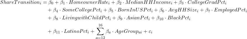
Where:
- i: neighborhood i.
- ShareTransitioni: share of renter (or homeowner) households that are likely to transition into homeowners (or renters) who currently reside in neighborhood i.
- AgeGroupai: share of population in age groups of: below 18, 18 to 24, 25 to 34, 35 to 44, 45 to 54, 55 to 64, and 65 and above in neighborhood i.
- β0: constant.
- εi: error term.
The regression analysis covers 256 neighborhoods out of 272 in Los Angeles County. Sixteen neighborhoods were excluded from the regression because we cannot obtain reliable socioeconomic indicators for them, or they have a very few number of renter and homeowner families due to their small populations. Those neighborhoods are: Chatsworth Reservoir, Elizabeth Lake, Green Valley, Griffith Park, Hansen Dam, Hasley Canyon, Lake Hughes, Lake Los Angeles, Littlerock, Ramona, Sepulveda Basin, Stevenson Ranch, Unincorporated Catalina Island, Universal City, Val Verde, and West San Dimas.
We ran alternative scenarios. First, we conducted sensitivity analyses using the 80th percentile as as a different cutoff to identify households likely to experience a housing transition. The results and main conclusions stayed consistent. We also tested a higher threshold—the 95th percentile—and found that the geographic distribution of likely transitioning households remained similar. Additionally, we re-ran the analysis using LABarometer’s OLS regression results. This produced similar overall spatial patterns, although the clustering effects were less pronounced.
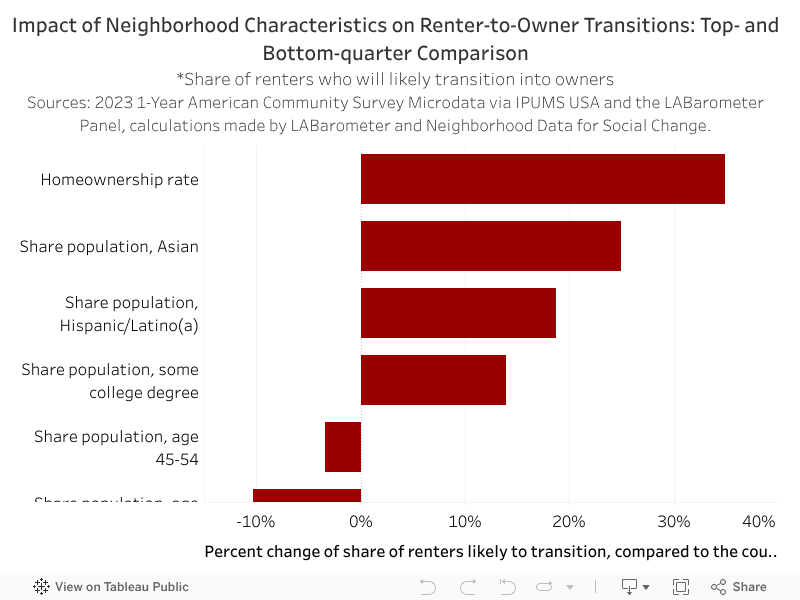
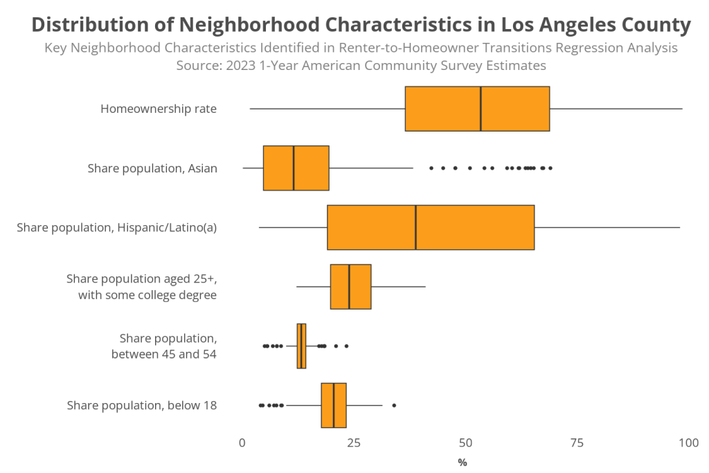
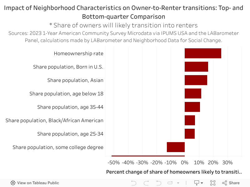
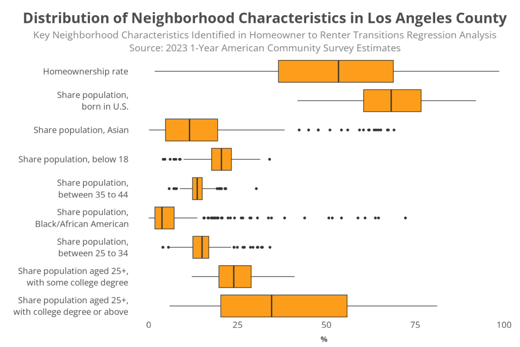
To quantify how changes in neighborhood characteristics influence housing transition patterns, we simulate what happens when a neighborhood moves from the 25th percentile (bottom quarter) to the 75th percentile (top quarter) for each trait. These calculations use the results from our analysis. Because these characteristics are distributed differently across neighborhoods, we use a box plot to display their typical ranges and help interpret these effects.
Let’s use the “share of Asian population” variable as an example. Our regression model found that, all else being equal, neighborhoods with a higher proportion of Asian residents tend to have more renters who are likely to become homeowners. Specifically, for this variable, the model calculates a coefficient of 0.170.
The box plot below shows the range of neighborhood characteristics that are statistically relevant in our estimations. Each box goes from the 25th percentile (left edge) to the 75th percentile (right edge) of the data. For context, if you compare a neighborhood at the 75th percentile for Asian population to one at the 25th percentile, the difference in renters likely to become homeowners is about 25% higher in the neighborhood with more Asian residents. Here’s how it is calculated:
- Take the difference in Asian population between the 75th and 25th percentile (19.412% – 4.743%).
- Multiply by the estimated coefficient (0.170).
- Divide by the average share of renters likely to move (≈10%).
Therefore: (19.412% – 4.743%) × 0.170 ÷ 0.10 ≈ 25%.
The full table of regression results, along with the distributions for each neighborhood characteristic is available in this methodology page. With this information, you can also reproduce the results in the figures.
Renter-to-Owner
Owner-to-Renter
Regression Outputs
Regression of the share of households likely to have a housing status transition on neighborhood-level demographic and socioeconomic characteristics
Characteristics by Housing Type Dashboard
Data Points
|
DataSet
|
Definition & Notes
|
Source
|
|---|---|---|
|
Characteristics of Renters, Homeowners & Houseless Angelenos: Race/Ethnicity
|
The racial and ethnic makeup (see categories in Quantitative Methods across Chapters) of the population by housing status: renters, homeowners, and people experiencing homelessness.
|
2023 American Community Survey 1-year estimates accessed via IPUMS (Population in Rental Housing, Owner-occupied housing and Total population) 2023 Greater Los Angeles Homeless Count (All unhoused, sheltered and unsheltered population)
|
|
Characteristics of Renters, Homeowners & Houseless Angelenos: Age
|
The age distribution (see categories in Quantitative Methods across Chapters) of the population by housing status: renters, homeowners, and people exp
|
2023 American Community Survey 1-year estimates accessed via IPUMS (Population in Rental Housing, Owner-occupied housing and Total population) 2024 Greater Los Angeles Homeless Count (All unhoused, sheltered and unsheltered population)
|
|
Median Household Income by Tenure
|
The middle value for household income in Los Angeles County, measured in 2023 dollars, disaggregated into households occupied by homeowners and renters. Income is defined as any money that a person earns from work, selling products or services, or any other streams such as Social Security payments, pensions, child support, public assistance, annuities, money derived from rental properties, interest and dividends, etc.
|
2023 American Community Survey 1-year estimates Table B25119
|
